
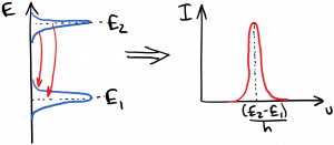
We’ve treated the spectra of light emitted by atoms transitioning between states 2 and 1 as having a single frequency $latex \nu = (E_2 – E_1) / h$, but of course that can’t be exactly true. The emission lines of atomic transitions have some finite spectral width, which is called line broadening; this broadening is caused by various broadening mechanisms.
You might reasonably wonder: if an electron transitions from state 2 to state 1, how can a photon be emitted with energy not exactly equal to the transition energy, and still conserve energy? The answer is that the atomic energy states themselves are broadened, as diagrammed below:
We’re going to define the lineshape function $latex g(\nu’) d\nu’$ as the probability that a spontaneously emitted photon will have a frequency in the range $latex \nu’$ to $latex \nu’ + d\nu’$. Since the emitted photon must have some frequency, the integral over all frequencies is 1:
$latex \displaystyle \int_0^{\infty} g(\nu’) d\nu’ = 1$
(Sorry for re-using the symbol g. We should always put $latex \nu$ next to this one to keep it separate from the degeneracy $latex g_2$ etc.) Incorporating the lineshape function, the updated spontaneous emission rate in some frequency range $latex \nu$ to $latex \nu + d\nu$ is $latex A_{21} N_2 g(\nu) d\nu$.
We could measure the lineshape function for a particular optical transition by observing the spontaneous emission spectrum of the light. The total optical power emitted by the atom in some frequency range $latex \nu$ to $latex \nu + d \nu$ is equal to $latex I(\nu) d\nu (Area)$, where $latex I$ here is the power per area per frequency, and $latex Area$ is the total surface area of some closed surface around the source. We can relate this to the updated spontaneous emission rate:
$latex \displaystyle I(\nu) d\nu (Area) = h \nu A_{21} N_2 g(\nu) d\nu (Vol)$
where $latex h \nu$ is the energy per photon, and $latex Vol$ is the total volume enclosed by the surface area on the left hand side.
Now we’re going to re-write our Einstein rate equations incorporating the lineshape function. Starting with spontaneous emission, we note that the rate equation for $latex N_2$ doesn’t depend on what the exact frequency of the emitted photon was; it only depends on whether a photon was emitted or not. Therefore we have
$latex \displaystyle \frac{dN_2}{dt} \biggr\rvert_{spon} = -A_{21} N_2 \int_0^{\infty} g(\nu’) d\nu’ $
$latex \displaystyle = -A_{21}N_2 $
so the total spontaneous emission rate is unchanged by including broadening.
We’ve already seen that the spontaneous emission, stimulated emission, and absorption rates are related to one another; therefore, we expect that the stimulated emission and absorption rates will also incorporate the lineshape function. However, when we consider stimulated emission and absorption, we have ‘external ‘ light interacting with the atom (i.e. light not emitted by that atom), and that light has its own energy spectral density $latex \rho(\nu)$. What we need to know is how well the external light’s spectrum overlaps with the lineshape function. If the two spectra did not overlap at all, then we would expect that the light wouldn’t interact with the atom at all, as diagrammed below:
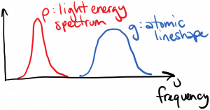
Note that g times $latex \rho$ is zero for all frequencies in this case.
If, on the other hand, the two spectra overlap strongly, then we expect strong interaction between the light and the atom:
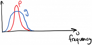
We measure the strength of this overlap by taking the product of the two spectra and integrating the result: $latex \int_0^{\infty} \rho(\nu’) g(\nu’) d\nu’$. For the two cases diagrammed above, you can hopefully convince yourself that the overlap integral will be zero in the first case, and large in the second case.
Incorporating the overlap integral into the stimulated emission and absorption terms, our updated rate equation for $latex N_2$ is:
$latex \displaystyle \frac{dN_2}{dt} \biggr \rvert_{radiative} = -A_{21} N_2 + B_{12} N_1 \int_0^{\infty} \rho(\nu’) g(\nu’) d\nu’ – B_{21} N_2 \int_0^{\infty} \rho(\nu’) g(\nu’) d\nu’ $
It is common with lasers in particular to have a situation where the spectral density of the light $latex \rho(\nu)$ has a much narrower spectral width than the lineshape function $latex g(\nu)$. This situation is diagrammed below.
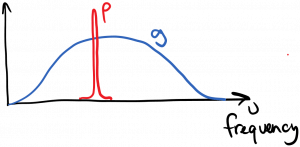
In this case, we can mathematically approximate $latex \rho(\nu’) \approx \rho_{\nu} \delta(\nu’ – \nu)$, where $latex \rho_{\nu}$ is the integrated optical energy per volume and is independent of frequency. Using this approximation allows us to evaluate the overlap integrals and the rate equation becomes:
$latex \displaystyle \frac{dN_2}{dt} \biggr \rvert_{radiative} = -A_{21} N_2 + B_{12} N_1 \rho_{\nu} g(\nu) – B_{21} N_2 \rho_{\nu} g(\nu) $
where $latex g(\nu)$ is the lineshape function evaluated at the frequency of the laser light.
The rate equation is just fine in this form, but sometimes you’ll see it written a bit differently, and I’ll show you how that happens here. For one thing we have that
$latex \displaystyle \rho_{\nu} = \frac{I_{\nu}}{c / n} $
where $latex I_{\nu}$ is the intensity (power / area) of the laser beam. Using this, and the Einstein relations, we can say
$latex \displaystyle \frac{dN_2}{dt} \biggr \rvert_{radiative} = -A_{21} N_2 – \left( A_{21} \frac{\lambda^2}{8 \pi} g(\nu) \right) \frac{I_{\nu}}{h \nu} \left[ N_2 – \frac{g_2}{g_1} N_1 \right] $
(Can you find stimulated emission and absorption in this expression?) The quantity in parenthesis is often defined as the stimulated emission cross-section, and has units of area:
$latex \displaystyle \sigma(\nu) = A_{21} \frac{\lambda^2}{8 \pi} g(\nu) $
So the rate equation becomes
$latex \displaystyle \frac{dN_2}{dt} \biggr \rvert_{radiative} = -A_{21} N_2 – \frac{\sigma(\nu) I_{\nu}}{h \nu} \left[ N_2 – \frac{g_2}{g_1} N_1 \right] $
You must be logged in to post a comment.