
As we’ve seen, in an inhomogeneously broadened laser far above threshold, multiple modes can lase simultaneously at different frequencies. Each lasing mode is amplified by a different subgroup of atoms, and doesn’t have any dependence on the other modes; therefore, the phase of each mode relative to the others is generally random. In a modelocked laser, we will take steps to ‘lock’ the phases of all the lasing modes so that they have a definite relationship to one another. The reason that this is desirable will be described below.
For a Fabry-Perot laser with mirror spacing L, the frequency separation between longitudinal modes in Hz is given by $latex c / 2 L$, which is the free spectral range. Therefore the angular frequency separation between longitudinal modes is $latex 2 \pi$ times the free spectral range, and we define this quantity as $latex \Omega$:
$latex \displaystyle \Omega = \frac{\pi c}{L} $
We’re going to assign some more symbols here, so we can do the math for a general case rather than a specific case. If we have $latex M$ lasing modes, each with their own frequency, let’s say $latex \omega_0$ is the lowest lasing mode (angular) frequency. The angular frequencies of the lasing modes would then be $latex \omega_0$, $latex \omega_0 + \Omega$, $latex \omega_0 + 2 \Omega$, and so forth up to $latex \omega_0 + (M – 1) \Omega$. Then we can write the total electric field inside the laser cavity at some fixed position (z = 0) as
$latex \displaystyle E_{tot}(t) = Re \left( \sum\limits_{m = 0}^{M -1} C_m \exp{(i [ (\omega_0 + m \Omega) t + \phi_m] )} \right)$
where $latex C_m$ is the amplitude of the $latex m^{th}$ mode, and $latex \phi_m$ is the initial phase of the $latex m^{th}$ mode. If the amplitudes $latex C_m$ and the phases $latex \phi_m$ are constant in time, the above total field is periodic in time with period $latex 2 \pi / \Omega$, because:
$latex \displaystyle E_{tot}(t + 2 \pi / \Omega) = Re \left( \sum\limits_{m = 0}^{M -1} C_m \exp{(i [ (\omega_0 + m \Omega) (t + 2 \pi / \Omega) + \phi_m]) } \right)$
$latex \displaystyle = Re \left( \sum\limits_{m = 0}^{M -1} C_m \exp{(i [ (\omega_0 + m \Omega) t + \phi_m] )} \exp{(i [2 \pi \omega_0 / \Omega + 2 \pi m])} \right)$
The quantity $latex \omega_0 / \Omega$ should be an integer representing the longitudinal mode number of the lowest-order lasing mode. Therefore the entire second exponential is 1, and we have
$latex \displaystyle E_{tot}(t + 2 \pi / \Omega) = E_{tot}(t)$
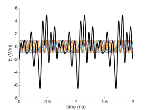
So the field is periodic in time if the amplitudes $latex C_m$ and phases $latex \phi_m$ are constant in time. For a fairly coherent laser we expect that the phases $latex \phi_m$ will be varying relatively slowly compared to the oscillation frequency; however, they are varying randomly with respect to one another, which leads to random fluctuations of the total field and intensity. For example, below we’ve plotted the individual mode fields (in various colors) and the total field (in black) for 10 modes with identical amplitudes $latex C_m = 1$ and random initial phases. You can see that the total field has a random-looking time dependence, which will evolve into different random-looking time dependences as the relative mode phases change over time.
Let’s imagine that instead we could lock all the mode phases $latex \phi_m$ to some constant value. For simplicity we’ll take all the $latex \phi_m = 0$. If we also have identical mode amplitudes $latex C_m = 1$ (which we won’t, in practice, but it’s a reasonable place to start) then our total field becomes:
$latex \displaystyle E_{tot}(t) = Re \left( \sum\limits_{m = 0}^{M -1} \exp{(i (\omega_0 + m \Omega) t)} \right)$
$latex \displaystyle = Re \left( \exp{(i \omega_0 t)} \sum\limits_{m = 0}^{M -1} \exp{(i m \Omega t)} \right)$
This is a geometric series, which we can evaluate. After some manipulation it becomes
$latex \displaystyle E_{tot}(t) = Re \left( \exp{(i \omega_0 t)} \exp{(i M \Omega t / 2)} \frac{\sin{( (M – 1) \Omega t / 2)}}{\sin{(\Omega t / 2)}} \right)$
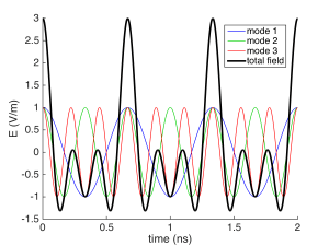
which looks like a periodic pulse train. We’ve plotted it first for 3 modes using L = 10 cm, which results in a period of $latex 2 \pi / \Omega = 2 L / c$ = 2/3 ns :
then five modes:

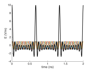
and finally 10 modes:
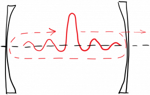
The advantage of modelocking, then, is that it produces a regular train of high-intensity pulses, which are useful for various applications. Note that the pulse period $latex 2 L / c$ is exactly the round-trip time of the laser. What this suggests is that there is a single pulse within the laser cavity, which is traveling back and forth between the mirrors at the speed of light. A portion of this pulse leaks out of the output-coupling mirror on each round trip. This is diagrammed below.
In order to achieve modelocking in practice, we work backwards from the knowledge of what a modelocked laser should produce – a periodic pulse train – and configure the cavity to encourage the formation of such a pulse train. In particular, we can modulate the losses (or the gain) in the cavity in such a way as to make a pulse train favorable. For example, suppose that we insert a component within the laser cavity which leads to increased optical loss (via absorption, or scattering, or whatever) whenever the pulse ISN’T present. When the pulse arrives, the loss decreases. This could take the form of a shutter which absorbs light when closed, and passes light when open. This shutter would have to be operated at a high frequency, as it must be opened and closed once every round trip time for the light.
In practice, making such a fast mechanical shutter is challenging. We may instead use an acousto-optic modulator, which diffracts light out of the beam when activated, and can be switched very fast. Alternatively, we may use a saturable absorber, which is a device that absorbs less light as the optical intensity increases. Another option is to pump the gain medium with another modelocked laser! The key is to modulate either the gain or the loss within the cavity at a frequency equal to the frequency separation between lasing modes. This generates sidebands for each mode, which exactly overlap with the neighboring mode frequencies, thus coupling the modes and locking their phases.
You must be logged in to post a comment.