ECE_2036_Lab_5.htm

ECE 2036 Lab
5                  Quantum Well Simulator

BACKGROUND

Many modern semiconductor lasers, such as the lasers used in
DVD and Blu-ray players, include one or more quantum wells in their active
regions (the regions that produce light). 
The design of a simple quantum well laser diode is shown here:

http://upload.wikimedia.org/wikipedia/en/4/42/Simple_qw_laser_diode.svg

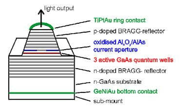
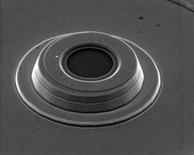
Below is a schematic and a scanning
electron micrograph of a vertical-cavity surface-emitting laser (VCSEL) with
multiple quantum wells:

        

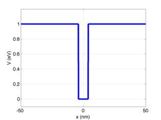
A quantum well is a very thin (usually less than 100
Angstroms thick) layer of material sandwiched between two layers of a different
material (called barriers).  For the
purposes of this lab we will use GaAs as the quantum
well material and AlAs as the barrier material.  The quantum well material is chosen to have a smaller bandgap energy than the
barriers.  The result of this is that the
quantum well forms an energy ‘well’ for electrons in
the layer, as diagrammed below:

where x is the spatial coordinate
and V is the potential energy of an electron. 
Electrons become trapped in the quantum well, and are more likely to
lose their energy and emit light of the desired wavelength (color), which is
the goal of laser design.  The well is so
thin that the electron behaves like a standing wave within the well.  (The wave behavior of electrons is one of the
major discoveries of quantum mechanics. 
This quantum mechanical behavior in the well leads to the name ‘quantum
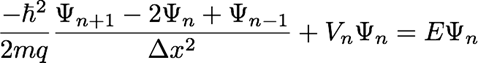
well’).  In steady state, the electron wavefunction obeys the time-independent Schrodinger
equation, which in one spatial dimension is given by:

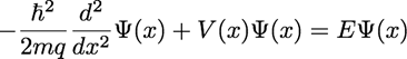
where ħ is the reduced Planck
constant, m is the mass of the electron, q is the charge of an electron, V is
the potential energy of the electron in electron-Volts (eV),
and E is the total energy of the electron in electron-Volts.  Ψ is the wavefunction
of the electron.  The Planck constant,
electron mass, and electron charge can be easily obtained from Google, just be sure to use MKS units.  Also, in our case we should use the EFFECTIVE
mass of electrons in GaAs, which is 0.067 times the
usual electron mass.  (The effective mass
is actually different in the AlAs barriers, but
that’s not a huge correction in our case).

The time-independent Schrodinger equation is an eigenvalue
equation.  There are many solutions for
the wavefunction Ψ  and energy E.  The wavefunction solutions
are called eigenfunctions of the equation, and each eigenfunction has a corresponding eigenvalue, which is its
energy E.  Physically, an eigenfunction and its eigenvalue represent an allowed state
for an electron in the quantum well.  By
calculating these eigenvalues and eigenfunctions, we
can predict the rate and wavelength of light emission from quantum well
lasers.  For example, as the energy E of
a state increases, the wavelength of light emitted by electrons occupying that
state will decrease (the light will become more blue, or ‘blueshift’).  The goal of this project is to calculate
states (eigenvalues and eigenfunctions) for electrons
in quantum wells.

In order to solve the Schrodinger equation on a computer, we
must discretize it – in other words, solve it on a grid.  A sample one dimensional grid is shown
below.  There are N total points in the
grid.

              x₁|_________x₂|_________x₃|_________…
_________x_n-1|_________x_n|_________x_n+1|_________
… _________x_N|

We will assume constant grid spacing, Δx
= x_n – x_n-1.  We want to calculate Ψ at every point on
the grid: Ψ(x_n)
= Ψ_n. 
We previously saw the finite difference approximation for a derivative,
and we can apply this approximation twice to derive a finite difference
approximation for a second derivative:

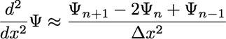
Inserting this approximation in the Schrodinger equation, we
have the discretized equation that we must solve:

We can write this as a matrix eigenvalue equation.  Define the following useful constant:

A=

 ħ2(2mqΔx2)

then our matrix eigenvalue
equation is:

(2A+V1)-A00⋯-A(2A+V2)-A0⋯0-A(2A+V3)-A⋯00-A(2A+V4)⋯⋮⋮⋮⋮⋱Ψ1Ψ2Ψ3Ψ4⋮=EΨ1Ψ2Ψ3Ψ4⋮

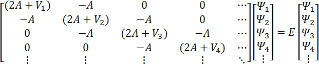
The large matrix on the left is called the Hamiltonian
matrix, and the column vectors are arrays representing the wavefunction.  Normally we’d have to worry about boundary
conditions, but in this case we’re assuming the wavefunction
goes to zero at the ends of our grid, so it takes care of itself.

Now the question is, how do we
solve this matrix eigenvalue equation on the computer?  There are many possible techniques.  The simplest is known as power
iteration.  In this approach, we take an
initial guess for the wavefunction, and we keep
multiplying it by the Hamiltonian matrix to generate a new wavefunction,
over and over again (iteratively).  Since
we don’t want our wavefunction to grow or shrink too
much, we normalize the new wavefunction after each
matrix multiplication.  If our initial
guess isn’t too terrible, our wavefunction will
eventually transform into the eigenfunction with the
largest eigenvalue.  (This works because
any arbitrary wavefunction – such as our initial
guess – is equal to the sum of all the eigenfunctions,
each multiplied by some amplitude.  Every
time we multiply the wavefunction with the
Hamiltonian, each eigenfunction in the sum is
multiplied by its corresponding eigenvalue. 
If we do this repeatedly, the eigenfunction
with the largest eigenvalue will grow the fastest and eventually dominate the wavefunction.)

In order to properly normalize the wavefunction,
we have to tell you what the physical meaning of the wavefunction
is.  The square of the wavefunction is the probability density of finding the
electron at various points in space.  In
other words, at places where the square of the wavefunction
is large, we are more likely to find the electron.  If we want to calculate the percent
probability of finding the electron in some region, we must integrate the
square of the wavefunction over that region:

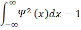
Probability of finding the electron between xa and xb=xaxbΨ2xdx

So, clearly the total probability of finding the electron
SOMEWHERE must be 1, and this is how we normalize the wavefunction:  we force the integral

-∞∞Ψ2xdx=1

To approximate this integral, we add up all the values in
our discretized wavefunction (column vector) and
multiply by the grid point separation, Δx:

n=1NΨn2∆x=1

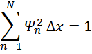
To ensure this summation is equal to one for our actual wavefunction, we divide our wavefunction
by the square root of this sum.  This is
called normalization:

Ψm,
normalized=Ψmn=1NΨn2∆x

We’re most interested in the lowest energy states (smallest
eigenvalues) in the well.  Unfortunately
power iteration gives us the LARGEST eigenvalues!  To resolve this, we just subtract a large
constant number from the potential energy V at every point.  This will make the smallest energies in the
well into the most negative (largest magnitude) energies, and power iteration
will find them for us.  I will take care
of this step for you, so you don’t need to worry about it until the time comes
to calculate eigenvalues.

What should we choose as our initial guess for the wavefunction?  All of
the potential energy profiles V you will solve in this lab are symmetric around
x = 0.  This means that some of the eigenfunctions will be even and others will be odd.  We expect the lowest energy state to be even
and the next higher state to be odd. 
Therefore, we will choose an even function as the initial guess for the
lowest energy state, and an odd function as the initial guess for the next
higher energy state.  Use a constant
function as your even initial guess, and a straight line as your odd initial
guess.

 

SUMMARY OF SOLUTION
STEPS FOR TWO LOWEST ENERGY EIGENFUNCTIONS

To summarize:  The
procedure to calculate the lowest energy quantum well states is as follows:

(1)  Read in the
spatial grid and V from an input file, and set up the Hamiltonian matrix

(2)  Create a wavefunction array equal to your initial guess for the
lowest energy eigenfunction (the zeroth
eigenfunction). 
Because we want an even initial guess, set each element of this wavefunction array equal to one

(3)  Update your wavefunction array to equal the Hamiltonian matrix times
your wavefunction array

(4)  Normalize your wavefunction array

(5) Repeat (iterate) steps (3) – (4) until your solution has
converged.  You can write a convergence
test if you want (ie. check to see that the wavefunction is no longer changing) but it is sufficient to
run 5000 iterations.

(6) Store your wavefunction array
as the solution for the zeroth eigenfunction.

(7) Set up a wavefunction array
equal to your initial guess for the next higher energy eigenfunction
( the first eigenfunction).  Because we want an odd initial guess, set
each element of this wavefunction array equal to the
corresponding spatial grid point (x grid point)

(8)  Repeat steps (3)
– (4) until your solution has converged, or 5000 iterations.

(9)  Store your wavefunction array as the solution for the first eigenfunction.

 

FINDING A HIGHER
ENERGY EIGENFUNCTION

We expect the next higher energy state after the first two
(the second eigenfunction) to be even, which makes it
harder to find, because the power iteration method will find the zeroth eigenfunction again if we
use an even initial guess.  But there is
a trick we can use to find the second eigenfunction.  We must find the zeroth
eigenfunction first, and store it, as described
above.  Then, we start over with an even
initial guess, but we add a step to each iteration.  At the start of each
iteration (steps (3) and (4) are a single iteration), we subtract off
the part of the wavefunction that resembles the zeroth eigenfunction.  (In principle we should only have to do this
once, but for various reasons it works better to do it after
each iteration.)  We do this by
taking an inner product between our trial wavefunction
and the eigenfunction we already found:

inner=n=1NΨn(eigenfunction0n)∆x

Multiply this by the zeroth eigenfunction, and then subtract that product from the
trial wavefunction:

Ψn,
orth=Ψn-inner*eigenfuncti��n0n

We can call this step ‘orthogonalization’.  After doing this we should multiply by the
Hamiltonian and normalize, as before.  So
our new iteration is: orthogonalize, multiply by
Hamiltonian, normalize, repeat.  We repeat these steps 5000 times, and store
the result, similar to above.  In this
way we can calculate the second eigenfunction.

In order to find eigenvalues, we note that multiplying the
Hamiltonian times an eigenfunction should produce the
same eigenfunction times its eigenvalue.  Therefore, in order to calculate the
eigenvalue,  find
a point where the eigenfunction is not zero (or very
small) and calculate eigenvalue = ((Hamiltonian * eigenfunction)
/ (eigenfunction)) using that point.

 

SAMPLE INPUT AND
OUTPUT

I provide a sample input file for a single quantum well
(sqw.csv).  The input file contains the x
grid and V for each point on the grid. 
The potential profile contained in that file is the same as shown above:

However, I’ve semi-arbitrarily subtracted 230 from V at each
point in order to force the lowest energy eigenvalue to be the largest in
magnitude (most negative).  Solving this
problem should produce the following output:

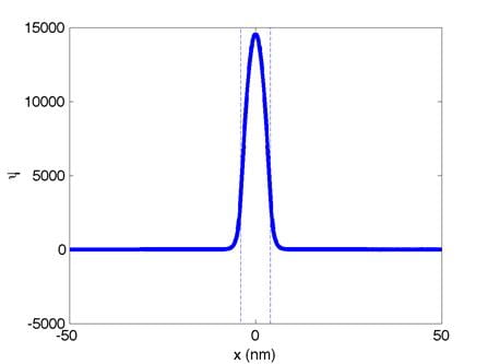
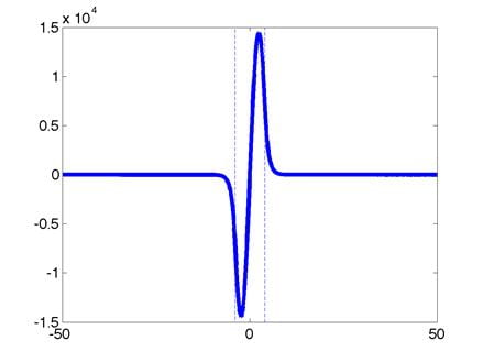
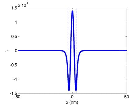
These are the normalized zeroth,
first, and second eigenfunctions, respectively.  (Don’t worry if your eigenfunctions
are upside down, a factor of -1 is not important here.)  The quantum well boundaries are indicated
with dashed lines.  The corresponding
eigenvalues are:

0^th:  E₀
= -229.94                            1^st:  E₁ = -229.75                             2^nd:  E₂ = -229.45

We would like to add 230 to these to undo the arbitrary
subtraction of 230 that I did earlier. 
If we ‘fix’ the eigenvalues in this way, we obtain:

0^th:  E₀
= 0.06 eV                            1^st:  E₁ = 0.25 eV                             2^nd:  E₂ = 0.55 eV

 

TASKS

Below I provide a skeleton code that reads in the input file
that you specify when you execute the program. 
For example, if you compile the skeleton code and name your executable a.out,
and at the command prompt type:

./a.out
sqw.csv

The program would read in sqw.csv.  The skeleton code includes a ‘Matrix’ class
and a constructor that initializes a matrix with zeros.  It also includes an ‘ActiveRegion’
class which contains V and the x grid. 
You must add various objects to the ActiveRegion
class, such as the Hamiltonian, which will be an object of the Matrix
class.  Also add the eigenfunctions
to the ActiveRegion class by calculating them.  You must also print out the eigenfunctions to comma-separated files.  You are required to overload at least one
operator, in order to multiply the Hamiltonian matrix and the wavefunction.

I also provide an input file that contains the x grid and
V(x) for three quantum wells (mqw.csv). 
V vs. x is plotted below:

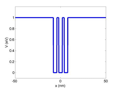
You must demonstrate the following using the mqw.csv input
file:

(A)  Calculate and
plot the zeroth eigenfunction
for mqw: 50 points

(B)  Calculate and
plot the first eigenfunction for mqw:
10 points

(C)  Calculate the zeroth and first eigenvalues for mqw:
20 points

(D)  Calculate and
plot the second eigenfunction for mqw:
10 points

(E)  Calculate the
probability that an electron in the zeroth eigenfunction of mqw will be
found in the center quantum well: 10 points

Please plot the eigenfunctions
using any plotting program of your choice (Matlab,
Excel, etc.) and bring your plots to your demonstration.  You should be prepared to plot the eigenfunctions using the output files generated by your
code and a plotting program if asked to do so by the TA.

Useful input/output files and skeleton code:

http://users.ece.gatech.edu/~bklein/2036/files_for_lab_5.zip